ML Last Term Notes

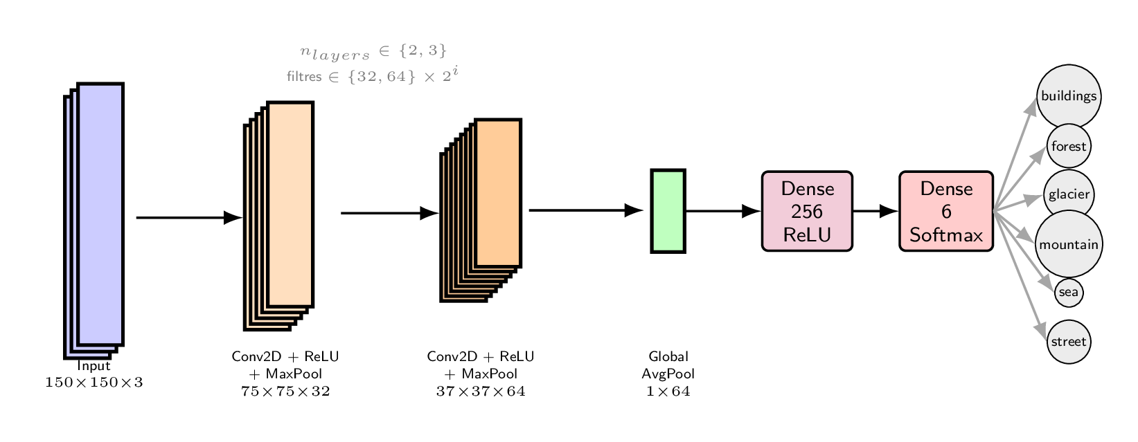
1. CNN Backpropagation

Extending gradient descent to update kernels and weights in a convolutional architecture. Gradients propagate through pooling and convolutional layers via the chain rule.

1.a Forward Pass Recap

Layer	Equation / Description
Convolution	$net_c = X * K$ — linear operation between input $X$ and kernel $K$
Detector	$H = \text{ReLU}(net_c)$ — non-linearity zeroing negative activations
Pooling	Max/Average pooling for dimensionality reduction and regularization
Fully Connected	$O = \text{Softmax}(H \cdot W + b)$ — final classification layer

1.b Backward Mechanism

Update FC Weights (W)

$\frac{\partial E}{\partial w_{ji}} = \frac{\partial E}{\partial o_j} \cdot \frac{\partial o_j}{\partial net_j} \cdot \frac{\partial net_j}{\partial w_{ji}}$

$\Delta W = -(\text{target} - \text{output}) \cdot \text{Output}(1-\text{Output}) \cdot H$

Update Kernel (K)

$\frac{\partial E}{\partial K} = \frac{\partial E}{\partial net_j} \cdot \frac{\partial net_j}{\partial H} \cdot \frac{\partial H}{\partial net_c} \cdot \frac{\partial net_c}{\partial K}$

Gradient propagates backward through Pooling → Activation (ReLU) → Kernel.

Max Pooling Backprop Gradient passes only to the max-value unit from the forward pass; all others receive zero gradient.

Parameter Count (Weight Sharing)

$\text{Params} = (\text{FilterW} \times \text{FilterH} \times \text{Channels} + 1) \times \text{NbFilters}$

Weight sharing makes CNNs far more parameter-efficient than FFNNs on the same input size.

---

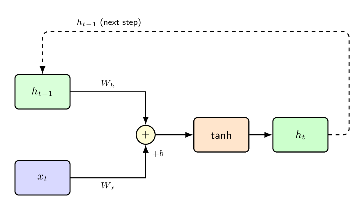
2. Recurrent Neural Networks (RNN)

A class of neural networks for sequential data where the order of inputs is crucial. RNNs maintain a hidden state that carries information across timesteps.

2.a Motivation: IID Breakdown & Sequential Data

Standard supervised learning assumes data samples are Independent and Identically Distributed (i.i.d.). Sequential data violates this — in language, time-series, or sensor readings each observation depends on previous ones. A vanilla FFNN has no mechanism to share context across positions, and requires fixed-size input.

RNN Solution A recurrent connection feeds the hidden state $h^{(t-1)}$ back into the computation at step $t$, encoding the sequence history into a running “memory” vector.

2.b Sequence Modeling Types

Type	Description	Example
One-to-One	Standard FFNN — single input → single output, no sequence	—
Many-to-One	Sequence input → single output	Sentiment analysis, time-series forecasting
One-to-Many	Single input → sequence output	Image captioning
Many-to-Many (Sync)	Input & output same length	POS tagging, NER, frame labeling
Many-to-Many (Delayed)	Encoder-Decoder: output starts after full input consumed	Machine translation

2.c Architecture & Forward Equations

$h^{(t)} = f_h\!\left(W_{xh}\, x^{(t)} + W_{hh}\, h^{(t-1)} + b_h\right)$

$o^{(t)} = f_y\!\left(W_{ho}\, h^{(t)} + b_{ho}\right)$

Where:

• $W_{xh}$: input→hidden, $W_{hh}$: hidden→hidden (recurrent), $W_{ho}$: hidden→output
• $f_h$: typically $\tanh$ — $f_y$: softmax (classification) or linear (regression)

2.d Multi-Layer RNN & Parameter Sharing

RNN cells can be stacked: the hidden state of layer $\ell$ becomes the input of layer $\ell+1$. In Keras, intermediate layers require return_sequences=True. The defining property is parameter sharing — the same $W_{xh}, W_{hh}, W_{ho}$ are used at every timestep, enabling variable-length inputs and efficient parameter use.

---

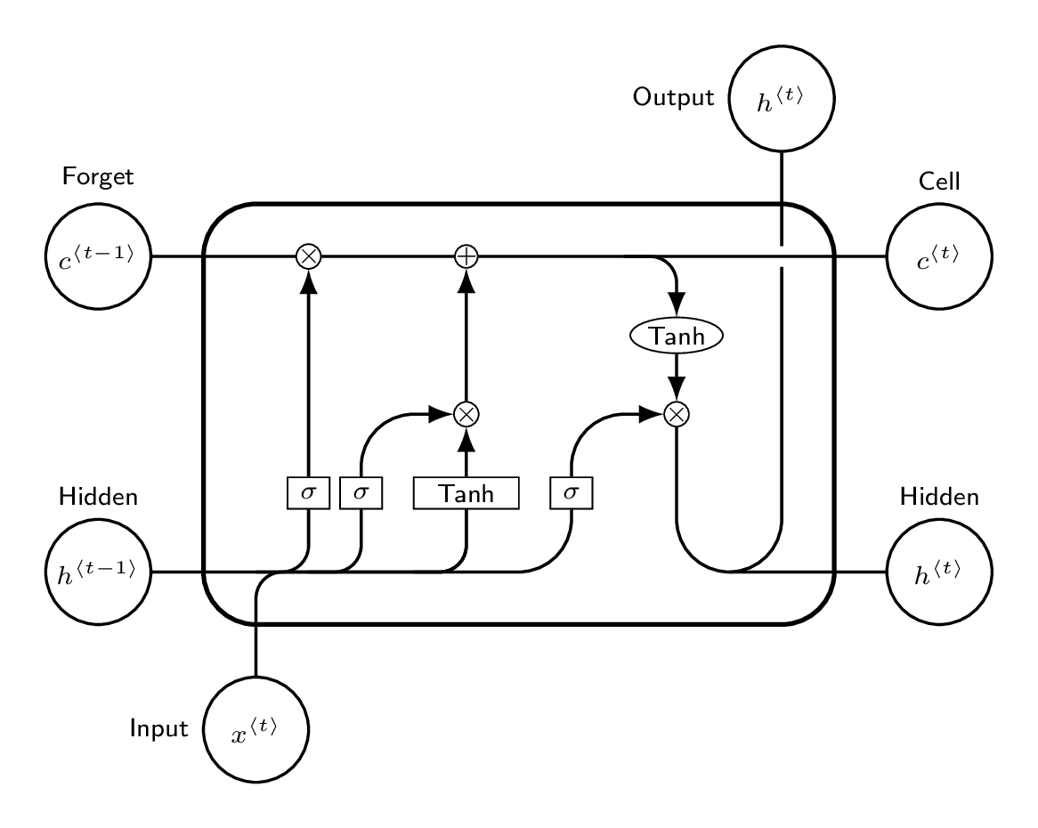
3. LSTM & Vanishing Gradient

LSTM was designed to solve the vanishing gradient problem in standard RNNs by maintaining a separate cell state — a gradient highway regulated by learnable gates.

3.a Vanishing Gradient Problem

During BPTT, gradients are multiplied repeatedly by $W_{hh}$ and $\tanh'(\cdot) < 1$. For long sequences this product approaches zero exponentially — the network cannot learn long-range dependencies. The cell state in LSTM keeps this product near 1 when the forget gate is open.

3.b Gate Equations

All gates receive concatenated input $[h^{(t-1)}, x^{(t)}]$:

$f_t = \sigma\!\left(W_f\,[h^{(t-1)}, x^{(t)}] + b_f\right) \quad\text{(Forget)}$

$i_t = \sigma\!\left(W_i\,[h^{(t-1)}, x^{(t)}] + b_i\right) \quad\text{(Input)}$

$\tilde{C}_t = \tanh\!\left(W_c\,[h^{(t-1)}, x^{(t)}] + b_c\right) \quad\text{(Candidate)}$

$o_t = \sigma\!\left(W_o\,[h^{(t-1)}, x^{(t)}] + b_o\right) \quad\text{(Output)}$

State Updates:

$C^{(t)} = \underbrace{C^{(t-1)} \odot f_t}_{\text{keep from past}} \;+\; \underbrace{i_t \odot \tilde{C}_t}_{\text{add new info}}$

$h^{(t)} = o_t \odot \tanh\!\left(C^{(t)}\right)$

$\odot$ = element-wise multiplication. $f_t \approx 1$ keeps old cell state; $f_t \approx 0$ forgets it.

Gate	Role
Forget $f_t$	$\sigma$ output 0 = forget old memory; 1 = keep entirely
Input $i_t$	Controls how much of the candidate $\tilde{C}_t$ is written to cell state
Candidate $\tilde{C}_t$	Proposed new values for cell state via $\tanh$ of concatenated input
Output $o_t$	Filters what fraction of $C^{(t)}$ is exposed as hidden state $h^{(t)}$

3.c Parameter Counting

Each gate has weight matrix shape $(m+n) \times n$ plus bias $n$, where $m$ = input dim, $n$ = LSTM units:

$\text{LSTM params} = (m + n + 1) \times 4n$

$\text{Total (+ output layer)} = (m + n + 1) \times 4n \;+\; (n + 1) \times k$

$m$ = input dim, $n$ = LSTM units, $k$ = output classes. Factor 4 = four gates (f, i, c̃, o).

---

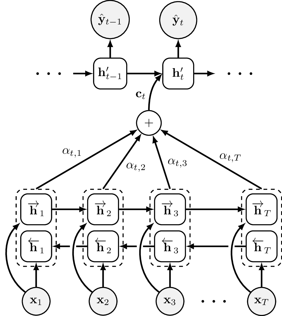
4. Attention Mechanism

Attention was introduced to overcome the information bottleneck of a fixed-length context vector in vanilla Encoder-Decoder networks. The decoder now dynamically focuses on different encoder positions at each decoding step.

4.a Encoder-Decoder Without Attention

The vanilla seq2seq model compresses the entire input sequence into a single fixed vector $c = h^{(T_x)}$. The decoder generates output from only this vector. For long sequences, this bottleneck causes severe information loss.

Bottleneck Problem For a 50-word sentence, all information must fit into one fixed-size vector. Empirically, translation quality degrades sharply as input length grows.

4.b Bahdanau (Additive) Attention

At each decoder step $t$, a different context vector $c_t$ is computed as a weighted sum over all encoder hidden states $\{h_j\}$:

$e_{tj} = v_a^\top \tanh\!\left(W_a\, s_{t-1} + U_a\, h_j\right) \quad\text{(alignment score)}$

$\alpha_{tj} = \frac{\exp(e_{tj})}{\displaystyle\sum_{k=1}^{T_x} \exp(e_{tk})} \quad\text{(attention weights via softmax)}$

$c_t = \sum_{j=1}^{T_x} \alpha_{tj}\, h_j \quad\text{(context vector)}$

$s_{t-1}$: previous decoder hidden state — $h_j$: encoder state at position $j$ — $W_a, U_a, v_a$: learned alignment params. Score computed before decoder step $t$ (uses $s_{t-1}$).

Alignment Matrix $\alpha_{tj}$ Visualizing all $\alpha_{tj}$ values reveals which source positions each output token attends to — giving interpretable word alignments in translation tasks.

4.c Luong (Multiplicative) Attention

Luong et al. compute the alignment score after the decoder step, using the current hidden state $h_t$:

$\text{score}(h_t, \bar{h}_s) = \begin{cases} h_t^\top \bar{h}_s & \text{dot} \\ h_t^\top W_a\, \bar{h}_s & \text{general} \\ v_a^\top \tanh\!\left(W_a\,[h_t;\, \bar{h}_s]\right) & \text{concat} \end{cases}$

	Bahdanau	Luong
Hidden state used	$s_{t-1}$ (pre-step)	$h_t$ (post-step)
Formula type	Additive	Multiplicative
Context scope	Many-to-one or many-to-many	Same

---

5. Self-Attention & Transformer

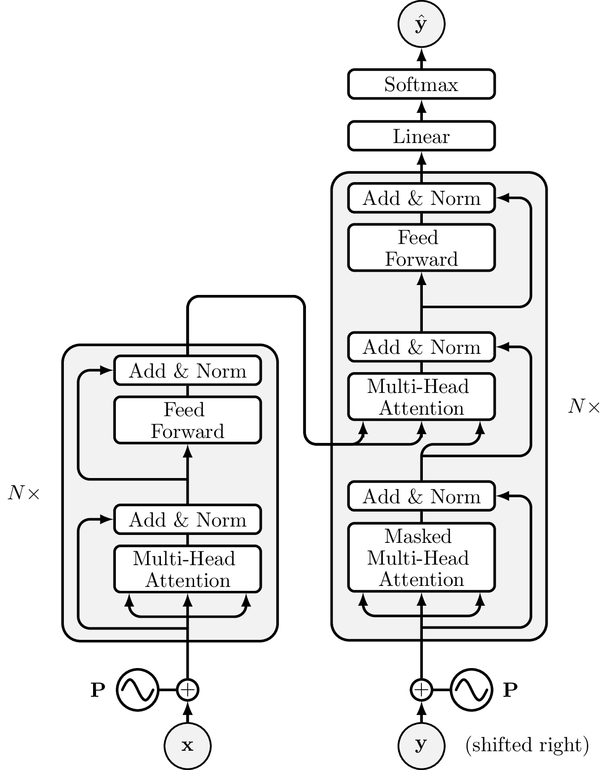
The Transformer (Vaswani et al. 2017) replaces recurrent cells with self-attention layers entirely, enabling fully parallel computation and direct long-range dependency modeling.

5.a Q / K / V Self-Attention

For input sequence $X = [x_1,\ldots,x_N]$, three linear projections create Query, Key, and Value vectors per position:

$q_n = \beta_q + \Omega_q\, x_n \quad\text{("what am I looking for?")}$

$k_m = \beta_k + \Omega_k\, x_m \quad\text{("what do I have?")}$

$v_m = \beta_v + \Omega_v\, x_m \quad\text{("what I contribute")}$

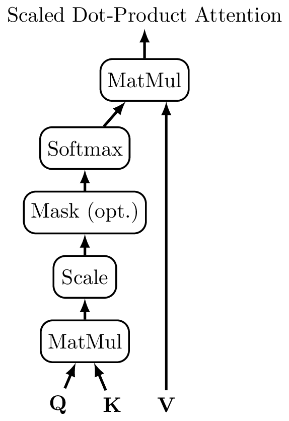
Scaled Dot-Product Self-Attention:

$a[x_m, x_n] = \text{softmax}_m\!\left[\frac{k_m^\top q_n}{\sqrt{D_q}}\right]$

$\text{Sa}[X] = V \cdot \text{Softmax}\!\left[\frac{K^\top Q}{\sqrt{D_q}}\right]$

Division by $\sqrt{D_q}$ prevents dot-products from growing large and saturating softmax. Each position receives a weighted sum of all value vectors.

5.b Transformer vs RNN Encoder-Decoder

	RNN	Transformer
Processing	Sequential: $h^{(t)}$ depends on $h^{(t-1)}$	All positions in parallel
Dependency path	$T$ steps between distant positions	$O(1)$ via self-attention
Positional info	Implicit in recurrent order	Explicit positional encoding (sinusoidal or learned)
Multi-head	—	$H$ independent heads; concatenate outputs

Why This Matters In an RNN, information from step 1 must survive $T{-}1$ transformations to reach step $T$. In a Transformer, every pair of positions attends to each other directly in a single layer — drastically reducing the path length for long-range information.

---

6. Backpropagation Through Time (BPTT)

BPTT trains recurrent networks by unrolling them into a deep feed-forward network (with shared weights), then applying standard backpropagation.

6.a BPTT Procedure

1. Forward — Compute all $h^{(t)}$ and $o^{(t)}$ for the full sequence.
2. Loss — Compute total loss $E = \sum_t E_t$ (e.g., cross-entropy at each output step).
3. Backward — Compute $\partial E / \partial W_{xh},\; \partial E / \partial W_{hh},\; \partial E / \partial W_{ho}$ by accumulating gradients across all timesteps (shared weights).
4. Update — Apply accumulated gradients via SGD / Adam to the shared weight matrices.

Truncated BPTT Backpropagation is limited to $k$ steps back for very long sequences. Reduces memory and computation at the cost of not learning ultra-long-range dependencies.

---

7. Reinforcement Learning

RL is a paradigm where an agent learns a policy through interaction with an environment, using reward signals as the only feedback. No labeled examples — the agent discovers good behavior via trial and error.

7.a RL vs Supervised Learning

	Supervised Learning	Reinforcement Learning
Input	Labeled pairs $(x, y)$	No labels; reward $R_t$
Feedback timing	Immediate, correct answer given	Delayed; reward may come much later
Actions affect future?	No	Yes — actions influence future states
Goal	Minimize prediction error	Maximize cumulative reward

Reward Hypothesis All goals can be described as maximizing the expected cumulative reward. Central hypothesis of RL.

7.b Agent-Environment Loop

At each timestep $t$: agent observes $S_t$, selects action $A_t$, environment returns reward $R_{t+1}$ and next state $S_{t+1}$.

$H_t = O_1, R_1, A_1,\; O_2, R_2, A_2,\; \ldots,\; A_{t-1}, O_t, R_t$

$S_t^a = f(H_t)$

Agent state is any function of the history. In fully observable environments $S_t^a = S_t^e$.

7.c Return & Discounted Return

Undiscounted:

$G_t = R_{t+1} + R_{t+2} + \cdots = \sum_{k=0}^{\infty} R_{t+k+1}$

Discounted:

$G_t = \sum_{k=0}^{\infty} \gamma^k\, R_{t+k+1}, \quad 0 \leq \gamma \leq 1$

$\gamma = 0$: only immediate reward. $\gamma \to 1$: all future rewards equally valued. Ensures sum converges; reflects that near-term rewards are more certain.

7.d Value Functions & Policy

$v(s) = \mathbb{E}\!\left[G_t \;\middle|\; S_t = s\right] \quad\text{(state-value)}$

$q(s,a) = \mathbb{E}\!\left[G_t \;\middle|\; S_t = s,\; A_t = a\right] \quad\text{(action-value)}$

$A = \pi(S) \quad\text{(deterministic)} \qquad \pi(A \mid S) = P(A_t = a \mid S_t = s) \quad\text{(stochastic)}$

Component	Description
Policy	Agent’s behavior function — maps states to actions or distributions
Value Function $v(s)$	Expected future reward from state $s$
Action-Value $q(s,a)$	Expected future reward from taking action $a$ in state $s$
Model (optional)	Predicts $S_{t+1}$ and $R_{t+1}$ given $S_t, A_t$ — not always learned
Model-Free	Learns from raw experience (Q-learning, SARSA)
Model-Based	Builds environment model to plan ahead

7.e Q-Learning & SARSA

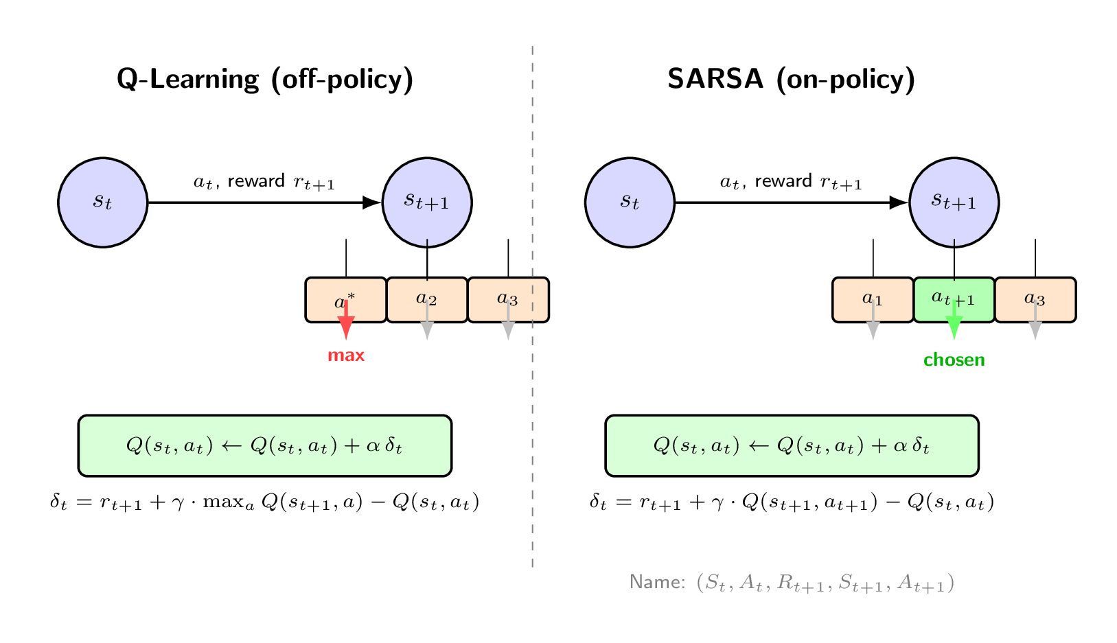
Both learn an action-value function $Q(s,a)$. The only difference is which next-step value is used as the bootstrap target:

Q-Learning (Off-Policy):

$Q(s_t, a_t) \leftarrow Q(s_t, a_t) + \alpha\,\delta_t$

$\delta_t = r_{t+1} + \gamma \cdot \max_{a}\, Q(s_{t+1}, a) - Q(s_t, a_t)$

Bootstraps from the greedy best action in $s_{t+1}$, regardless of what was actually taken. Learns optimal policy even while exploring.

SARSA (On-Policy):

$Q(s_t, a_t) \leftarrow Q(s_t, a_t) + \alpha\,\delta_t$

$\delta_t = r_{t+1} + \gamma \cdot Q(s_{t+1}, a_{t+1}) - Q(s_t, a_t)$

Bootstraps from the value of the next action actually chosen by the current policy.

SARSA Name Origin The update uses the tuple $(S_t,\, A_t,\, R_{t+1},\, S_{t+1},\, A_{t+1})$ — five elements, hence “SARSA”.

	Q-Learning	SARSA
Type	Off-policy	On-policy
Bootstrap target	$\max_a Q(s',a)$	$Q(s', a')$ where $a'$ is actually taken
Behavior	Optimistic — assumes best future action	Conservative — penalizes risky explorations
Convergence	To $Q^*$ regardless of exploration policy	To optimal for current exploration strategy
Differ when	$a_{t+1} \neq \arg\max_a Q(s_{t+1},a)$	Same condition

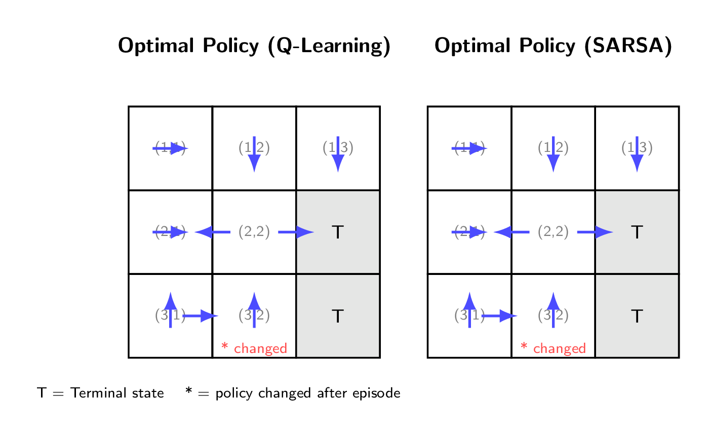
7.f Optimal Policy & Grid World

After training, $\pi^*$ selects $\arg\max_a Q(s,a)$ in each state. A single episode updates only visited states — the rest remain unchanged.

Episode Example Path $(2,1) \to (2,2) \to (3,2) \to (3,3)$ with $\alpha=0.5,\, \gamma=0.7$. Only $Q((2,1),R)$, $Q((2,2),D)$, $Q((3,2),R)$ are updated. Policy at $(3,2)$ changes from ”↑ or →” to ”↑ only” because $Q((3,2), R)$ falls sharply from reward $-10$.

---

8. Glossary

Term	Definition
IID	Independent & Identically Distributed — standard ML assumption violated by sequential data
Parameter Sharing	Same weight matrices $W_{xh}, W_{hh}, W_{ho}$ used at every RNN timestep
Vanishing Gradient	Gradients shrink exponentially during BPTT; solved by LSTM cell state highway
Cell State	LSTM long-term memory highway — regulated by forget / input gates
Context Vector	$c_t = \sum_j \alpha_{tj} h_j$ — weighted sum of encoder states used by decoder
Alignment Score	$e_{tj}$ measures relevance of encoder position $j$ to decoder step $t$
Self-Attention	Computes pairwise relationships between all token pairs in parallel
Q / K / V	Query, Key, Value — three learned linear projections in Transformer self-attention
Scaled Dot-Product	$\text{Sa}[X] = V \cdot \text{Softmax}[K^\top Q / \sqrt{D_q}]$
Return $G_t$	$\sum_{k=0}^\infty \gamma^k R_{t+k+1}$ — cumulative discounted reward from step $t$
Value $v(s)$	$\mathbb{E}[G_t \mid S_t = s]$ — expected return from state $s$
Policy $\pi$	Agent’s behavior; deterministic $A=\pi(S)$ or stochastic $\pi(A\|S)$
Q-Learning	Off-policy TD: bootstraps from $\max_a Q(s',a)$ — converges to $Q^*$
SARSA	On-policy TD: bootstraps from $Q(s',a')$ where $a'$ is actually taken
TD Error $\delta_t$	$r_{t+1} + \gamma\,Q(s_{t+1},\cdot) - Q(s_t,a_t)$ — correction signal for both algorithms

---

Goodfellow et al. (2016) · Hochreiter & Schmidhuber (1997) · Bahdanau et al. (2015) · Vaswani et al. (2017) · Sutton & Barto (2018) · IF3270 Lecture Decks 5–9 · Attention & Transformer diagrams: Fraser Love, NNTikZ (2024)